New methods for trajectory integration in Geant4

Report on Google Summier of Code 2017 project, May 30 - August 29, 2017

Dmitry Sorokin, MIPT

August 29, 2017

Work supervised by John Apostolakis, CERN

Work supported by Google as part of Google Summer of Code 2017, in the “CERN and HEP Software Foundation” umbrella organisation.

Introduction

In accelerator and detector simulation an application must emulate the tracks of charged particles. In the presence of an electromagnetic field, charged particles feel the Lorentz force, and, as a result, undertake curved trajectories. These can be described as an initial value problem (IVP), over a vector y :

where the vector y spans position, momentum and potentially polarisation variables, and the independent variable x can be either time or length along the curve.

If the field is not uniform the tracks are computed by numerically solving the above equation. In the simulation of High Energy Physics (HEP) experiments the field is typically evaluated by table lookup and interpolation. This makes function evaluations  expensive. So for simulation of complex experiments with a large number of tracks we need robust and time-efficient integration methods.

Challenges for the chosen methods/algorithms:

• Very large number of track segments (steps) in each simulation, taking a substantial fraction of the total simulation time (in the region of 10-20%);
• very robust integration of a variety of equations (with a user provided field) for different length scales, without any failures;
• high cost of field evaluation;
• change of momentum (currently only at end of a ‘physical’ step) due to interactions.  This imposes some limit on the ability to reuse previous derivatives (multi-step methods);
• need to find the intersection point between a curved trajectory and the surfaces of the experiment (or other user’s) volumes - which we seek to address using RK methods with interpolation to provide arbitrary intermediate points;
• observed that the step size sometimes oscillates, leading to the idea to try different step-size control methods.

This year’s GSoC project is dedicated to exploring a number of methods new to the Geant4 toolkit: new step-size control algorithms, steppers for oscillatory problems, and the introduction of integration ‘drivers’ that can make use of the FSAL property of existing RK steppers or alternative integration methods (Bulirsch-Stoer, developed in GSoC 2016.) The latter development also paves the way for the future use of interpolation for the progress of tracking and for volume intersection.

Part 1: New methods for step size control

Context

For nonuniform field right hand side (RHS) of the equation of motion can change significantly in one region (e.g. in a strong and/or quickly varying magnetic field) and slightly in a different region, e.g. one which has a weaker or slowly varying field. To integrate accurately in the regions with strong RHS changes, the integration must use a very small integration steps which will slow down integration in the regions with small RHS changes, if the step size is kept fixed.

To solve this problem the preferred methods involve adaptive step size control. Step size control algorithms adjust the step size dynamically to satisfy a chosen error tolerance (TOL). In this way the step size can be small enough in regions with strong field changes, and large in regions with small field changes.

The original step size control algorithm used in Geant4 is the one recommended in Numerical Recipes in C [4]:

where is the step size at iteration ,  is error estimation at iteration .  The parameter k depends on the order of the integration method used:  for successful steps () and for failed ones ().  

For mildly-stiff IVPs, when stability restricts the stepsize, frequent rejections of the stepsize may occur. This results in wasted function evaluations. It is possible to modify the stepsize control algorithm (but not the integration method) to prevent the oscillations.

An alternative stepsize control algorithm that is proposed by Gustafsson [1] is:         

where parameter controls the speed of convergence of the step size control algorithm and parameter controls the stability of the algorithm. The value of the parameter should be in the interval  where  is the parameter of the ‘standard’ step-size control algorithm. If  the Gustafsson step size control algorithm becomes the ‘standard’ algorithm.  The parameters should be chosen with special attention due to the tradeoff between the stability and the response time, and can be different for each integration algorithm.

The work done

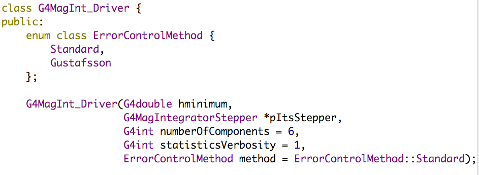
The new error control method has been implemented in the existing class G4MagInt_Driver. The user can choose which algorithm to use via optional parameter in the class constructor.

Results

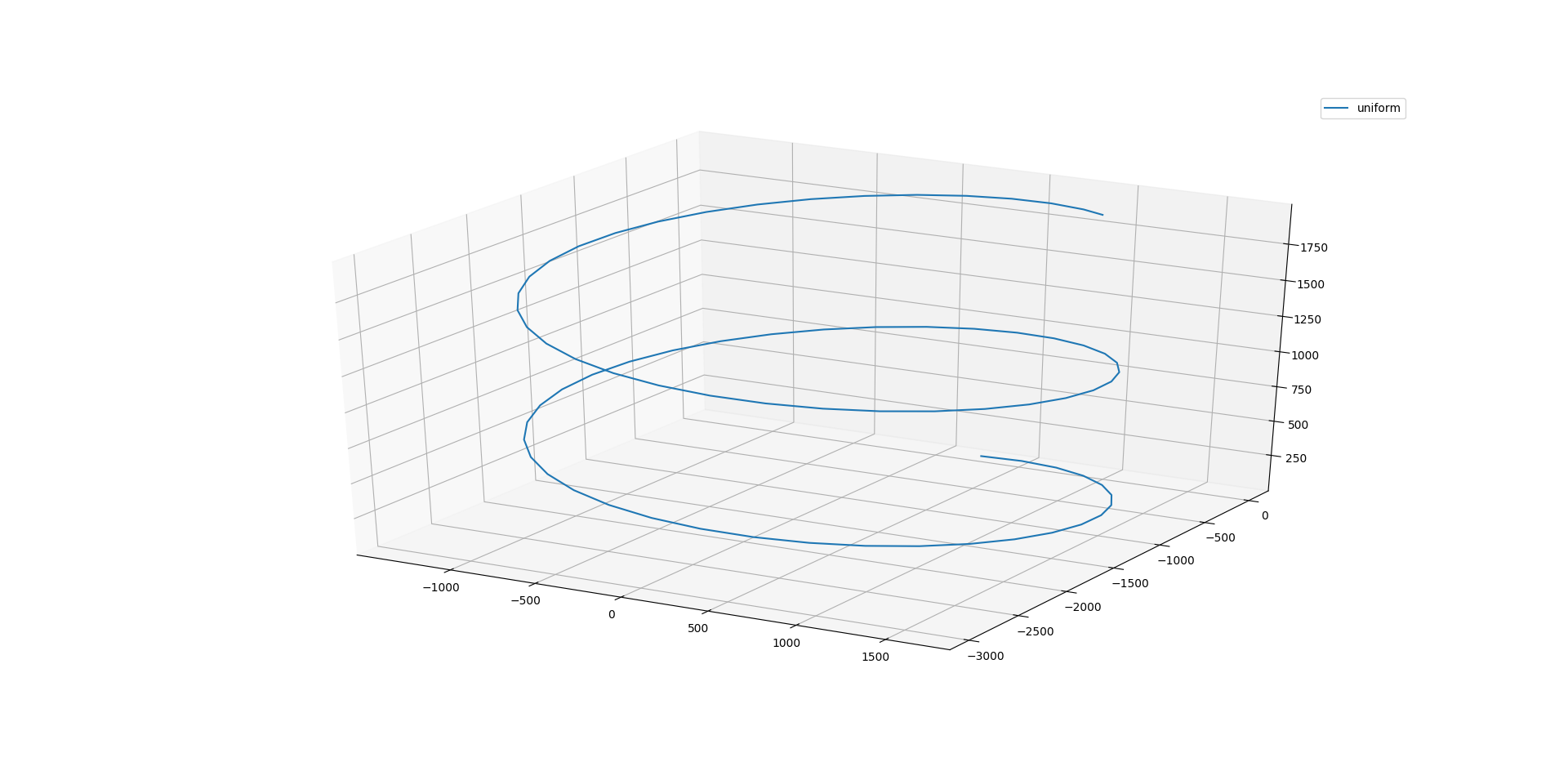
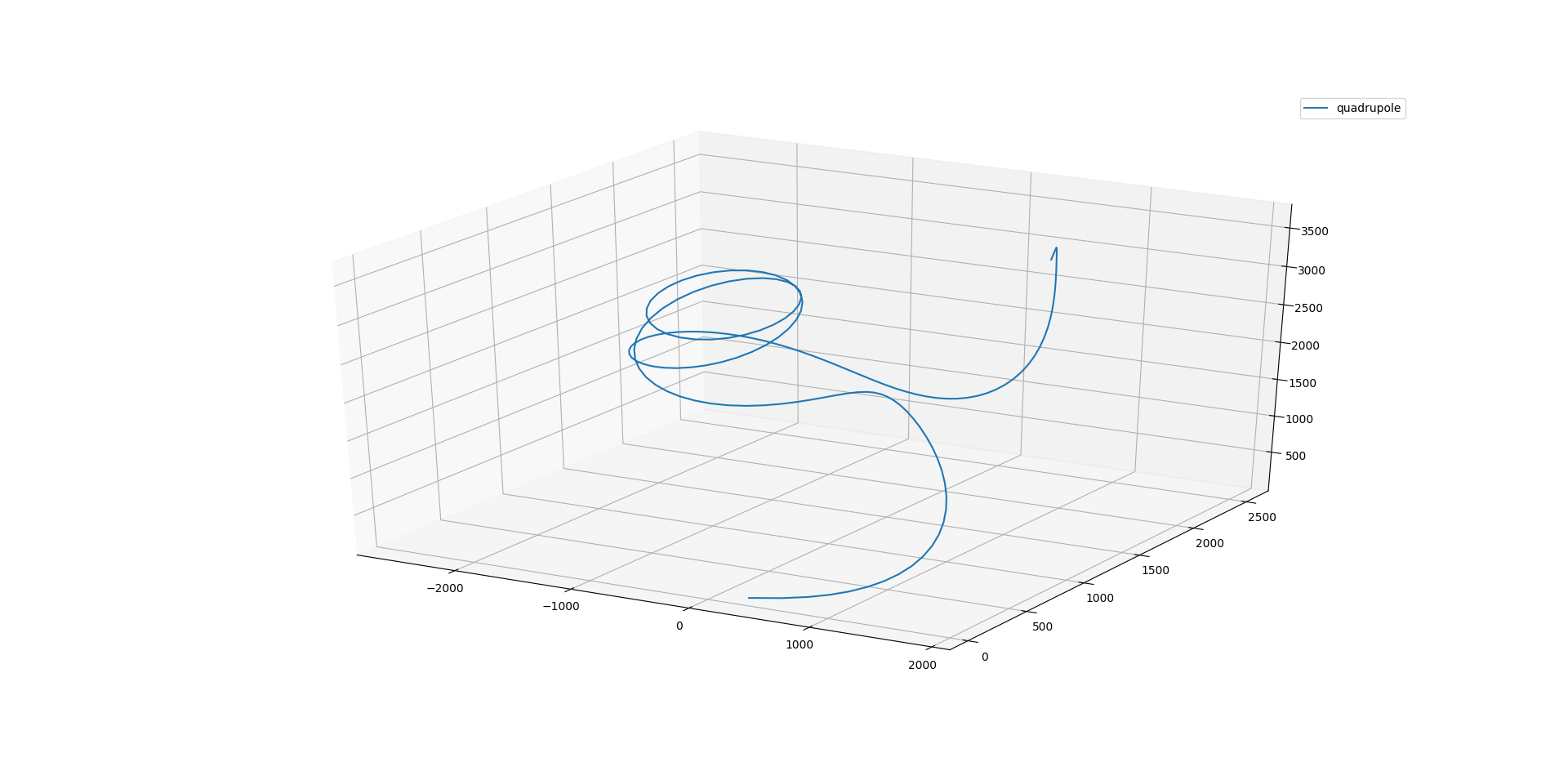
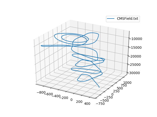
New step size control algorithm was tested in uniform, quadrupole and CMS magnetic fields. The tracks are in the figures below.        

Fig. 1. Tracks in the uniform, quadrupole and CMS magnetic fields.

In this tests no step size oscillations was observed. Gustafsson driver performed nearly the same as standard Runge-Kutta driver.

The main integral test to check the overall performance of the simulation which is used in this report is test NTST. It simulates the inner detector of the Babar experiment, with the realistic interpolated Babar field. Sample events are sample Babar events using the Pythia 6 event generator.

Number of field evaluations in the NTST test are presented in the table below. It is seen that the new algorithm is slightly more efficient.

Table 1. Number of calls to field per event in the NTST test. Stepper is G4DormandPrince745

The new algorithm is more efficient for the (c)  simulation, which is the most time consuming because it includes secondary charged particles with lower energies. It remains to be confirmed whether this is due to a higher probability of step size oscillations.

Part 2: Methods adapted for oscillatory problems

Context

• Franco [3] describes adapted Runge-Kutta methods. In the methods coefficients of Runge-Kutta methods are modified in such way that the method become accurate for oscillatory solutions. The coefficients depend on the parameter:

        ,

        where  is the main frequency of oscillations and t is the time step. That parameter  

        for pure magnetic field (B) can be calculated as:

,

        where h is the step size (length), q is the charge of the particle, p is the momentum

magnitude of the particle, and B is the strength of the field.

Results

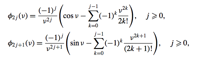
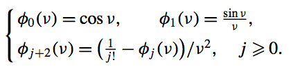
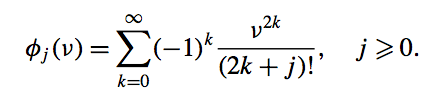
• In the article [3] coefficients of the adapted method are calculated using Bettis functions of parameter . Article [3] presents several options to calculate the Bettis functions:

• Explicit formulas

• Recursive formulas

• Taylor series

I have done benchmarks of the above three options and option four when the formula of needed Bettis function (i.e. j = 4) was precalculated. Time benchmarks are in the table 2 below.

Table 2. Time benchmarks of different implementation of the Bettis functions with  = 0.1. Time in milliseconds. Number of runs per formula is 1e7.

It is seen from the table 2 that explicit formula has the worst execution time. Taylor series is fast enough but it is accurate only for relatively small parameters . Execution times of the recursive formula and precalculated formula does not differs by much. For this reason we decided to use the recursive formula for large values of ,  and the Taylor series for the small ones.

Results for the NTST test are presented in the table 3 below. It is seen that implemented adapted classical RK4 method (ARK4) is about 16 percent more efficient that the classical RK4 method.

Table 3. Test NTST, number of field evaluations per event for G4ClassicalRK4 stepper and ARK4 stepper (adapted for oscillatory solutions classical RK4 stepper)

Part 3: Using FSAL in integration

Revising the integrator design

The Geant4 toolkit has contains the following three key classes for integration:

1. Stepper base class (G4MagIntegratorStepper)

2.   Driver (G4VIntegrationDriver - base class)

3.  ChordFinder (G4ChordFinder)

The roles of these different classes are the following:

• The Stepper class undertakes one integration step, incrementing an array of state variables, estimating their integration errors, and, optionally, estimating the distance between the midpoint of the curved trajectory and the chord between the starting and ending point.
• The Driver class uses the stepper object to integrate the equation of motion with adaptive step size control.
• The ChordFinder class uses the Driver object to integrate the equation of motion over steps satisfying a chord criterion.

A new abstract driver class  (G4VIntegrationDriver) was introduced In order to cope with the varying needs and capabilities of different classes of steppers, and the alternative Bulirsch-Stoer integration method (developed as part of the author’s 2016 GSoC project),

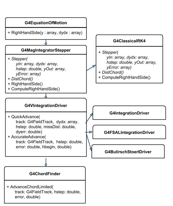
The new classes and their associations are represented in the UML diagram below.

Fig. 2. Uml diagram of the magneticfield package..

The addition of the new abstract driver base class has been used to create three new driver algorithms: one for the Bulirsch-Stoer multi-step integration scheme, and two for Runge Kutta integrators, one for FSAL RK methods and the other for non-FSAL methods.

The overhead of a large number of calls to virtual function is an issue in the overall performance of the integration process. To reduce the number of virtual calls the new driver classes are templated on the type of the stepper. This eliminates the virtual function call to the stepper methods, and also allows the use of steppers which don’t inherit from the stepper base class.

The original (G4MagInt_Driver) integrator is maintained for compatibility. It does not depend on the exact type of Stepper, allow the stepper to be changed during simulation and other capabilities of the existing (old) interface.

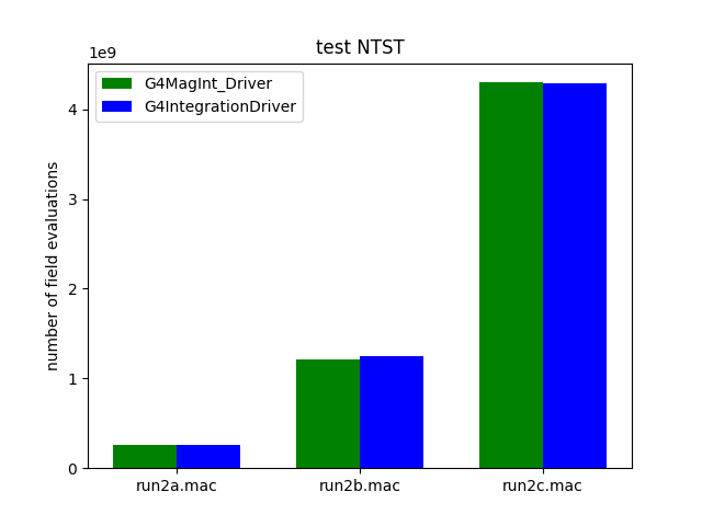
Fig. 3. Number of calls to field in the NTST test for G4MagInt_Driver and G4IntegrationDriver classes.

To confirm that the new classes work correctly we checked the number of calls to field in the NTST test, for both the original G4MagInt_Driver and the new template class G4IntegrationDriver. We note that G4IntegrationDriver uses the same step size control algorithm. As seen in figure 3, the number of field evaluations is very close.  

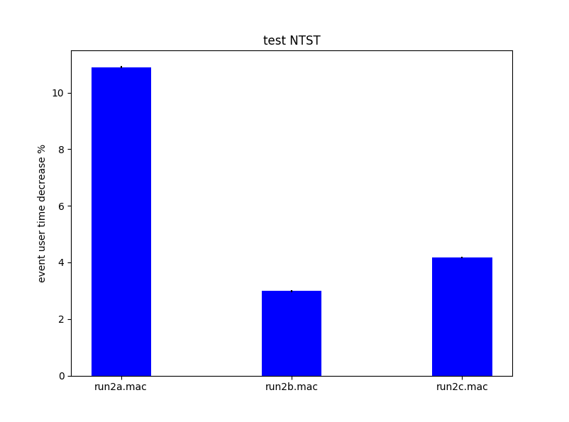
Fig. 4. Event user time decrease for the G4IntegrationDriver relative to G4MagInt_Driver class.

The results of a first performance benchmark (using ClassicalRK4 and 1,000 events) shown in figure 4 demonstrate that template driver implementation (G4IntegrationDriver) is a bit faster than G4MagInt_Driver. Performance is increased by 10% for run2a.mac, 3% for run2b.mac and 4% for run2c.mac. Further performance evaluation will seek to refine these measurements.

Implementation of new FSAL steppers with improved equilibrium states

Context

• A Runge-Kutta method has a First Same As Last (FSAL) property If the last stage is evaluated at the same point as the first stage of the next step. 
• Using this property one can get one RHS evaluation ‘for free’.  

The work done

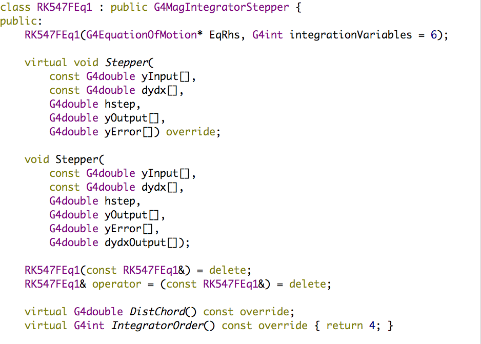
Current design of a FSAL stepper:

The RK547FEq1 stepper can be applied as FSAL and non-FSAL stepper. Because we created the template FSAL driver class we don’t need to add an additional base driver class for the FSAL steppers.

Higham and Hall [2] presented three FSAL Runge-Kutta steppers with stable equilibrium properties . These steppers were implemented as RK547FEq1, RK547FEq2, and RK547FEq3 with the interface described above and tested.

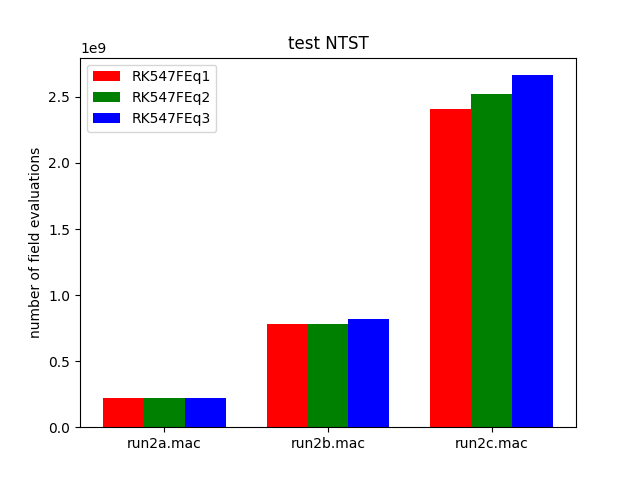
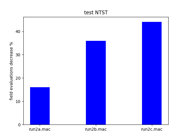
Fig. 5. Number of field evaluations for RK547FEq1,   Fig. 6. Field evaluations decrease for

           RK547FEq2, RK547FEq3 in test NTST.                      RK547FEq1 in comparison with

                                                                   Classical RK4.

From the Fig.5 it is seen that RK547FEq1 which has an near optimal error term is a bit more efficient method than the other two.

RK547FEq1 is more efficient than the ‘default’ stepper G4ClassicalRK4 method in number of field evaluations (Fig.6). Field evaluations decrease is 16%, 36%, 44% for run2a.mac, run2b.mac and run2c.mac accordingly.

Using the FSAL property of a method provides the derivative at the endpoint of a successful step.  Thus it saves one field evaluation at each good step. In case of seven stage method (RK547FEq1) this property can give up to 1/7  14% decrease in number of field evaluations. This is an upper bound estimate because it doesn’t take into account either failed steps, or processes (scattering, energy loss) which change the momentum and can also shift the final position of the particle, and thus reset the integration process. ( Further improvement could be made by explicitly saving the value of the field at the endpoint of a step, which could be used in the first evaluation of a subsequent step. In many cases such caching is already done inside the field class. )

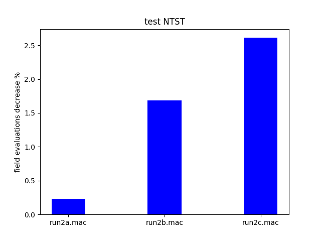
To evaluate the improvement in practice we used the same stepper (RK547FEq1) in both FSAL and non-FSAL ‘mode’ by using the corresponding driver classes.  The results in figure 7 demonstrate the decrease seen in the number of field evaluations for FSAL version - compared to the non-FSAL version. The maximal decrease seen is about 2.5% percent.

We note that this decrease is limited because the new G4FSALIntegrationDriver class uses the FSAL property only in the AccurateAdvance method. We will investigate using this property also in the QuickAdvance method in the future, as this will require changes in G4ChordFinder class.

Fig. 7. The decrease in the number of field evaluations for the new RK547FEq1 stepper when its FSAL property is used (the estimate of the final derivative is reused if valid), in comparison with its use when it’s FSAL property is not used.

Links

Branch for different step size control algorithms

Branch for template driver class

Branch for methods adapted for oscillatory problems

dev branch (all stable developments)

Appendix

Table 4. Test NTST, stepper G4ClassicalRK4, driver G4MagInt_Driver

Table 5. Test NTST, stepper G4ClassicalRK4, driver G4IntegrationDriver

Table 6. Test NTST, stepper ARK4, driver G4IntegrationDriver

Table 7. Test NTST, stepper RK547FEq1, driver G4IntegrationDriver

Table 8. Test NTST, stepper RK547FEq2, driver G4IntegrationDriver

Table 9. Test NTST, stepper RK547FEq3, driver G4IntegrationDriver

Table 10. Test NTST, stepper RK547FEq1, driver G4FSALIntegrationDriver

Table 11. Test NTST, stepper RK547FEq2, driver G4FSALIntegrationDrive

Table 12. Test NTST, stepper RK547FEq3, driver G4FSALIntegrationDriver

Table 13. Test NTST, stepper G4DormandPrince745, driver G4IntegrationDriver

References        

1. K. Gustafsson, “Control theoretic techniques for stepsize selection in explicit Runge-Kutta methods,” ACM Trans. Math. Softw., vol. 17, no. 4, pp. 533–554, Dec. 1991.                                                        
2. D. J. Higham and G. Hall, “Embedded Runge-Kutta formulae with stable equilibrium states,” J. Comput. Appl. Math., vol. 29, no. 1, pp. 25–33, Jan. 1990.        
3. J. Franco, “Runge–Kutta methods adapted to the numerical integration of oscillatory problems,” Appl. Numer. Math., vol. 50, no. 3–4, pp. 427–443, Sep. 2004.         
4. William H. Press, Saul A. Teukolsky, William T. Vetterling, Brian P. Flannery, Numerical recipes in C : the art of scientific computing. 2nd edition, 1992.